How to Draw a Plane in Matlab

Determining Stability using the Nyquist Plot

Contents

Statement of the Trouble
The Nyquist Path (no poles on jω axis)
The Nyquist Path (with poles on jω axis)
Counting Encirclements
Stability Margins

Statement of the Trouble

Given a single loop feedback system

we would like to be able to determine whether or non the airtight loop system, T(due south), is stable. This is equivalent to asking whether the denominator of the transfer function (which is the characteristic equation of the system)

has any zeros in the right one-half of the s-plane (recall that the natural response of a transfer function with poles in the right half plane grows exponentially with time).

If we perform a mapping (as explained on the previous page) of the function "1+L(due south)" with a path in "southward" that encircle the unabridged right one-half plane and we count the encirclements of the origin in the "ane+L(s)" domain in the clockwise management we get the number N=Z-P (where Z is the number of zeros, and P is the number of poles). What we desire, though, is Z, the number of zeros in the correct half airplane. But since nosotros know L(due south), we can easily find P, the numbers of poles of "1+L(s)." This is because any pole of L(s) is also a pole of "1+L(s)." So now nosotros know North (from the mapping) and we know P (from L(southward)), so we can easily determine Z.

Earlier continuing we brand one small change. Instead of mapping from "due south" to "1+50(s)" and counting encirclements of the origin, nosotros map from "south" to "L(s)" and count encirclements of the indicate -1+j0 in the circuitous airplane. This is because the origin in "1+Fifty(s)" corresponds to the "-1+j0" point in "50(s)" (if L(s)=-one, and so 1+Fifty(s)=0).

Key Concept: Statement of the Problem

To decide the stability of a organization we:

First with a system whose characteristic equation is given by "ane+L(south)=0."
Make a mapping from the "s" domain to the "L(s)" domain where the path of "south" encloses the unabridged correct one-half plane.
From the mapping we find the number N, which is the number of encirclements of the -1+j0 point in "L(southward)."
Annotation: This is equivalent to the number of encirclements of the origin in "1+L(s)."
We can factor 50(south) to determine the number of poles that are in the right one-half aeroplane.
Since we know N and P, we can determine Z, the number of zeros of "1+L(s)" in the right one-half plane (which is the aforementioned as the number of poles of T(south)).
If Z>0, the arrangement is unstable.

The Nyquist Path (with no poles on the jω axis).

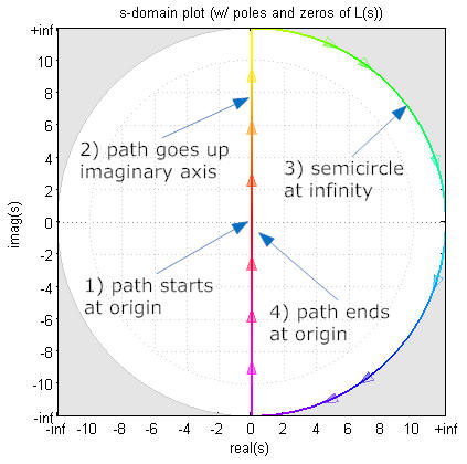
In the previous section, nosotros specified that the path of s should enclose the unabridged right half plane. To start, we assume that the function L(s) has no poles on the jω axis. We ascertain the path every bit starting at the origin, moving up the imaginary axis to j∞, following a semicircle (in the clockwise management), and then moving up the -jω axis and ending at the origin. This is shown below.

Let's examine this procedure with a couple of examples (followed by a video of the two examples). A multifariousness of examples follow on the next page (Examples).

Example: Nyquist path, no poles on jω axis, stable

Consider a arrangement with found Grand(s), and unity gain feedback (H(s)=1)

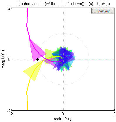
If nosotros map this office from "southward" to "L(s)" with the variable southward following the Nyquist path we get the following image (note: the image on the left is the "Nyquist path" the image on the right is called the "Nyquist plot")

If we zoom in on the graph in "L(southward)"

the start thing we detect is the multiple arrowheads at the origin. This is considering every bit the path in "s" traverses a semicircle at ∞ the path in "L(due south)" remains at the origin, but the angle of Fifty(due south) changes. More importantly, we can run into that it does non encircle the -1+j0, and then N=0. We too know that P=0, and since N=Z-P, Z is also equal to zero. This tells u.s. that the arrangement is stable. And, if we close the loop, we notice that the characteristic equation of the airtight loop transfer function is

which has roots at -two±17.2j so the system is indeed stable. Recall that the roots of the characteristic equation are the poles of the transfer function.

Beliefs of the Nyquist path when |s|→∞

A very large segment of the path in "southward" occurs when |s|→∞, shown every bit the large semicircle in the south-domain plot (i.e., the left plot). Nevertheless, during this segment of the plot, the path in 50(south) volition not movement, bold Fifty(s) is a proper transfer part. The order of the numerator polynomial of a proper transfer part is less than or equal to that of the denominator. Let's consider, start, the instance when the order of both polynomials is equal to n:

If |s|→∞, then the highest order term of the polynomial dominates and we become

And so, when |due south|→∞ the path in L(due south) is at a single point. (Annotation: In the Nyquist diagrams, since in that location are several arrowheads on the path in "s" as information technology makes it excursion at infinity, there are besides several arrowheads at this single bespeak in "L(s).")

If the loop gain, L(s), is strictly proper (i.e., the order of the numerator is less than that of the denominator)

and then

and the path in L(s) is at the origin while |s|→∞.

Instance: Nyquist path, no poles on jω axis, unstable

Consider the previous organization, with a sensor in the feedback loop

If we map this function from "s" to "L(south)" with the variable due south following the Nyquist path we become the post-obit image

We can run into that this graph encircles the -1+j0 twice in the clockwise direction so North=two. Nosotros as well know that P=0, and since N=Z-P, we tin summate that Z=2. This tells us that the organization is unstable, because the feature equation of the closed loop transfer role has two zeros in the right half plane (or, equivalently, the transfer role has two poles there). Nosotros can check this by closing the loop to get the characteristic equation of the closed loop transfer role:

which has roots at due south=-vii.5 and south=1.26±eight.45j so the system is indeed unstable with ii poles in the right one-half plane.

Video: Mapping with no poles on the jω axis

1 infinitesimal video created with the Matlab script NyquistGui

The Nyquist Path (with poles on the jω axis).

If there are poles on the jω axis, we can no longer use the Nyquist Path as specified above because the path will go through poles of Fifty(s) where its value is undefined. To handle that state of affairs we make small "detours" around the poles that are on the axis. These detours are small semicircles in the counterclockwise direction around these poles (so that the path stays in the right one-half plane), However, we make the radius of the detours infinitesimally small-scale, then they don't exclude any part of the right one-half aeroplane. For instance if we have

The path at present makes pocket-sized semicircular detour of infinitesimally modest radius around the poles at s=±j4. However, considering the path is and so shut to the pole, the magnitude of the path in "L(s)" is at infinity. And because the path is going around the pole in the counterclockwise direction in "southward" the path in "L(south)" is in the clockwise direction. This is shown beneath (in this diagram the radius of the detours is exaggerated so they tin can exist seen on the graph).

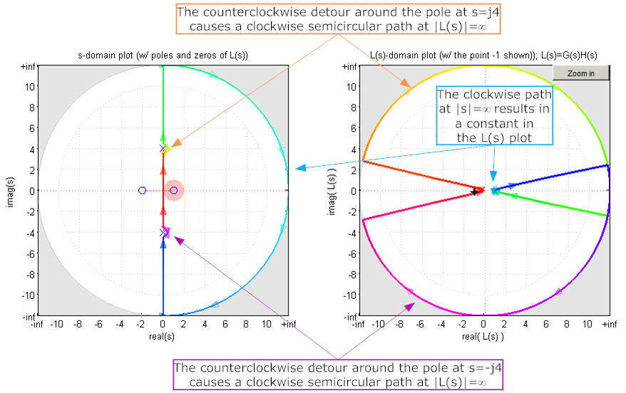
Note that:

The counterclockwise detours effectually the poles at s=±j4 results in a clockwise semicircle at Fifty(southward)=∞ in "L(s)" (meet video below)
The clockwise semicircle at infinity in "s" corresponds to a single point in "L(southward)"
If the counterclockwise detour was around a double pole on the axis (for instance two poles at the origin), the path in L(s) goes through an angle of 360° in the clockwise direction.

Again, we can double check this by finding the zeros of the feature equation.

This has roots at southward=-0.25±j2.63, so the arrangement is stable.

Video: Mapping with poles on the jω axis

ane½ infinitesimal video created with the Matlab script NyquistGui

Cardinal Concept: Detours around poles on the jω centrality

If the path in "s" makes a 180° counterclockwise detour around a pole on the jω axis, then the corresponding path in "50(south)" has space radius and goes through 180° in the clockwise direction. If the detour in "due south" is around two coincident poles (eastward.thou., 2 poles at the origin) the bending in "L(s) will be 360°.

Counting Encirclements

Counting the number of encirclements of the -one+j0 point is obviously of critical importance to determining the stability of the system (the number of encirclements in the clockwise management is the "North" in the equation "N=Z-P"). At that place are two means to exercise this. The start is easier conceptually, the 2nd is easier practically.

Counting encirclements by visualization

Imagine y'all are presented with the Nyquist diagram below

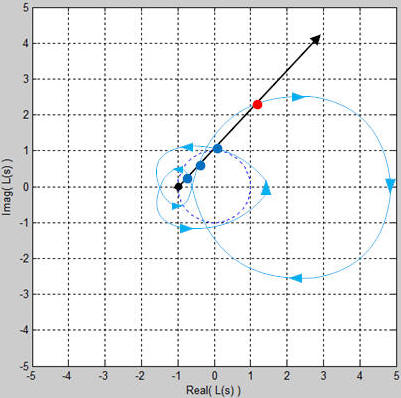
How many encirclements of the -i+j0 betoken are there. To visualize the reply, assume y'all accept a pointer whose base is at the -ane+j0 point and whose caput is anywhere on the Nyquist plot. For example nosotros can start at the point near the origin and call this angle zero (Note: since we volition exist traversing the unabridged path the identify where we start on the graph is arbitrary.)

We follow the path with the tip of our arrow to the first crossing of the jω axis (180° counterclockwise) and continue following the path until we get back to the starting point. As nosotros do so we proceed runway of the total bending that has been swept out by the arrow, equally shown beneath.

1) 180° counterclockwise	2) 0° (total)	3) 180° clockwise (full)	iv) 0° (total)

This diagram show 180° movement, ccw	Here nosotros have 180°, cw, for a total of 0°	Some other 180° cw, for a total of 180°, cw	A final 180° movement ccw yields 0° total.

When we are finished we have traversed a net of 0°, so the -1+j0 point is not encircled.

Notwithstanding, with a slightly dissimilar Nyquist diagram we get a different result. Start as earlier,

and so follow the path with our arrow

1) 180° counterclockwise	2) 360° ccw	3) 360° ccw


4) 360° ccw	5) 540° ccw	6) 720° ccw

In this case we have two encirclements in the counter clockwise direction.

Counting encirclements the easy fashion

An easier way to determine the number of encirclements of the -1+j0 indicate is to simply draw a line out from the point, in any directions. Consider the first example from higher up, shown below with a vertical line drawn from -1+j0.

If you count the number of times that the Nyquist path crosses the line in the clockwise direction (i.eastward., left to right in the image, and denoted by a red circumvolve) and decrease the number of times it crosses in the counterclockwise management (the blue dot), you get the number of clockwise encirclements of the -ane+j0 point. A negative number indicates counterclockwise encirclements. In the image in a higher place, at that place is one crossing in each direction, and therefore zero encirclements (equally determined previously).

The direction of the line draw is arbitrary. The paradigm beneath shows the same Nyquist path, simply a different line. In this case at that place are two clockwise crossings (red) and two counterclockwise crossings, for a total of cipher encirclements, as expected.

We now apply this technique to another example (the 2nd case from higher up), in which we have the same path shifted to the right.

Hither we run across two counterclockwise crossings of the line and hence two counterclockwise encirclements of -1+j0.

If nosotros choose a different line we get i clockwise crossing of the line, and iii counterclockwise crossings. Hence we have ii counterclockwise encirclements of -1+j0, every bit expected.

Gain and Stage Margins

At this point y'all may well enquire, "Why go through this whole procedure if nosotros can but find the airtight loop transfer part and encounter if it is stable?" The reason we use the Nyquist Stability Criterion is that it gives use information about the relative stability of a organization and gives us clues equally to how to make a system more stable. In particular, there are two quantities, the gain margin and the phase margin, that tin can be used to quantify the stability of a system.

A stable arrangement

Consider a system with

Let usa draw the Nyquist plot:

If we zoom in, we can see that the plot in "50(due south)" does not encircle the -1+j0, so the system is stable.

Nosotros tin verify this by finding the roots of the feature equation

The roots are at s=-5.5 and southward=-0.24±2.88j so the system is stable, as expected.

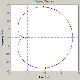
This can exist seen even more clearly using Matlab's "nyquist" command. In fact, the "nyquist" command is generally more useful for examining the details of a Nyquist plot (called here the Nyquist diagram) than the plots we have been using, but the plots we have been using may exist better for learning nearly the plots.

Now lets describe a unit circle effectually the origin (using Matlab'south "ltiview" command).

There are two spots on the Nyquist plot that are emphasized. The commencement is where the Nyquist plot crosses the existent centrality in the left half plane. If we zoom in and put the cursor over this point we become the following image.

As y'all can meet, the plot crosses the existent axis at near -2/3, or -0.67. This tells the states that if nosotros multiply 50(s) by a number greater than three/two that the path would encircle the -1+j0 and the systems would be unstable. So the "proceeds margin" is 3/2 or 20log₁₀(iii/2)=3.5dB. The greater the gain margin, the more stable the system. If the gain margin is zero, the arrangement is marginally stable. (Note: the text also shows that the Nyquist plot crosses the real axis when the Nyquist path is going through the point due south=j3.32 (this is the "frequency" shown).)

The 2nd point shows where the Nyquist plot crosses the unit circle as displayed on the images below.

The bending between between the betoken at which the plot crosses the unit circle (when the Nyquist path is at south=j2.73) has an angle of 14° to the horizontal axis. This tells us that if we decrease (where a subtract moves the plot in the clockwise direction) the phase of L(s) by more 14° that the -1+j0 signal becomes encircled and the arrangement becomes unstable. We say that the organisation has a stage margin of xiv°. A higher phase margin yields a more stable system. A phase margin of 0° indicates a marginally stable system. Notation: if you lot know about the frequency response time delays, recall that a fourth dimension delay corresponds to a change in phase - for this organisation nosotros could have a delay of 0.089 seconds (corresponding to 14° at 2.73 rad/sec). If you don't know about time delays, you can skip this.

A marginally stable system

If we multiply L(due south) by 3/2 we get

and we meet that the system gain and phase margins go to zero so we wait the organisation to be marginally stable.

We can verify this by finding the roots of the feature equation

The roots are at s=-6 and south=±3.32j so the system is marginally stable, as expected.

An unstable organisation

If we multiply the original L(s) by 4 we get

and we see that the system proceeds and phase margins become negative and so we expect the system to be unstable.

Nyquist Plot		Zoomed with negative proceeds margin shown		Zoomed with negative phase margin shown

The margins tell us that we'd have to decrease the gain past -8.52dB (multiply by 0.375) or change the phase past -25.9° to brand this organization stable. (Annotation: we tin readily verify the proceeds margin because we know that multiplication of L(south) by 3/2 made the organization marginally stable, and 4·0.375=3/ii (the current gain (4) multiplied by the gain margin (0.375) yields the gain that creates marginal stability (three/2).) We tin verify that the system is unstable by finding the roots of the characteristic equation

The roots are at due south=-7.5 and s=+0.75±four.64j so the organization is unstable, every bit expected.

Bated: Gain and Phase Margins may be Infinite

Infinite Gain Margin

The gain margin of a system will be infinite if the phase of the loop gain never reaches -180° (i.e., if the Nyquist plot never crosses the real axis in the left half aeroplane). If then the Nyquist path is every bit shown

The gain margin is infinite considering the path never crosses the real centrality in the left half aeroplane (the path goes to the origin as |southward|→∞.

Space Phase Margin

The phase margin will exist infinite if the magnitude of gain of L(s) is never greater than one. If then the Nyquist path is equally shown

The phase margin is infinite considering the gain is always less than one, so no affair how much the phase changes, the -1+j0 signal will never be encircled.

References

brantleysatepas.blogspot.com

Source: https://lpsa.swarthmore.edu/Nyquist/NyquistStability.html